Formula and function

Formula and function

In this lesson, we introduce you to basic rules for creating formulas and using functions. We feel one of the best ways to learn is through practice, so we provide several examples and explain them in detail. The topics we will cover include:

 

• rows and columns
• example math function: SUM()
• operators
• operator precedence
• example financial function: PMT(), loan payment
• using a “string” function (“string” is shorthand for “string of text”) inside a formula and nesting functions

Formulas are a mixture of “functions,” “operators,” and “operands.” Before we write a few formulas, we need to create a function but before we can create a function, we first need to understand row and column notation.

Rows and Columns

To understand how to write formulas and functions, you need to know about rows and columns.

Rows run horizontally and columns run vertically. To remember which is which, think of a column holding up a roof – columns go up-down and thus rows go left-right.

Columns are labeled by letters; rows by numbers. The first cell in the spreadsheet is A1 meaning column A, row 1. The columns are labeled A-Z. When the alphabet runs outs, Excel places another letter in front: AA, AB, AC… AZ, BA, BC, BC, etc.

Example: Function Sum()

Now let’s demonstrate how to use a function.

You use functions by typing them directly in or using the function wizard. The function wizard opens when you either pick a function from the “Formulas” menu from the “Function Library.” Otherwise, you can type = in a cell and a handy drop-down menu will allow you to pick a function.

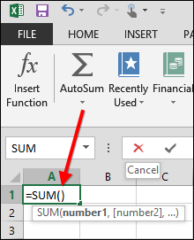
The wizard tells you what arguments you need to provide for each function. It also provides a link to online instructions if you need help understanding what the function does and how to use it. For example, if you type =sum into a cell, the in-line wizard shows you what arguments are required for the SUM function.

When you type a function, the wizard is inline or right at your fingers. When you select a function from the “Formulas” menu, the wizard is a pop-up box. Here is the pop-up wizard for the SUM() function.

For our first function, let’s use SUM(), which adds a list of numbers.

Suppose we have this spreadsheet to contain plans for budgeting your family’s vacation:

To calculate the total costs you could write =b2+b3+b4+b5 but it’s easier to use the SUM() function.

In Excel, look for the symbol Σ at the top left-hand corner of the Excel screen to find the AutoSum button (mathematicians use the Greek letter Σ for adding a series of numbers).

If the cursor is below the family budget numbers, Excel is smart enough to know that you want to sum the list of numbers above where you placed the cursor, so it highlights the numbers.

Press “enter” to accept the range selected by Excel or use the cursor to change which cells are selected.

If you look at what Excel put into the spreadsheet you can see that it wrote this function:

In this formula, Excel sums the numbers from B2 to B9. Note, we left some room below row 5 so that you could add to the family vacation budget – the cost will certainly go up as the kids list of what they want to do and where they want to go grows longer!

Math functions do not work with letters, so if you put letters into the column the result is shown as “#NAME?” as shown below.

#NAME? indicates that there is some kind of error. It could be any number of things including:

• bad cell reference
• using letters in math functions
• omitting required arguments
• spelling function name wrong
• illegal math operations like division by 0

The easiest way to select the arguments in a calculation is to use the mouse. You can add to or remove from the list of arguments to the function by enlarging or making smaller the box that Excel draws when you move the mouse or click in another cell.

We have clicked on the top of the square drawn by Excel to take “airline tickets” out of the budget. You can see the cross-hair symbol that you can draw to make the selected range larger or smaller.

Press “enter” to confirm the results.

Calculation Operators

There are two types of operators: math and comparison.

Math Operator	Definition
+	addition
–	subtraction, or negation, e.g., 6 * -1 = -6
*	multiplication
/	division
%	percent
^	exponent, e.g. 24 = 2 ^ 4 = 2 * 2 * 2 * 2 =16

There are other operators not related to mathematics like “&” which means concatenate (join end-to-end) two strings. For example, =“Excel” & “ is Fun” equals “Excel is Fun”.

Now we look at comparison operators.

Comparison Operator	Definition
=	equals, e.g., 2=4 or “b” = “b”
>	greater than, e.g., 4 > 2 or “b” > “a”
<	less than, e.g., 2 < 4 or “a” < “b”
>=	greater than or equal to – another way to think of this is >= means either > or =.
<=	less than or equal to.
<>	not equal to, e.g., 4<>6

As you can see above, comparison operators work with numbers and text.

Note, if you enter =”a”>”b” into a cell it will say “FALSE” since “a” is not greater than “b.” “b” comes after “a” in the alphabet, so “a” > “b” or “b” > “a.”

Operator Order Precedence

Order precedence is an idea from mathematics. Excel has to follow the same rules as mathematics. This topic is more complicated, so take a breath and let’s dive in.

Order precedence means the order in which the computer calculates the answer. As we explained in Lesson 1, the area of a circle is πr2, which is the same as π * r * r. It is not (πr)2.

So you have to understand the order precedence when you write a formula.

Generally, you can say this:

1. Excel first evaluates items in parentheses working inside out.
2. It then uses the order precedence rules of mathematics.
3. When two items have the same precedence, Excel works left to right.

The precedence of math operators is shown below, in descending order.

( and )	When parentheses are used, they override the normal rules of precedence. This means that Excel will do this calculation first. We explain this further below.
–	Negation, e.g., -1. This is the same as multiplying a number by -1. -4 = 4 * (-1)
%	Percent, means multiply by 100. E.g., 0.003 = 0.3%.
^	Exponent, e.g., 10 ^ 2 = 100
* and /	Multiply and divide. How can two operators have the same precedence? It just means that if a formula has two more operators with the same precedence, then the calculation is done left to right.
+ and –	Addition and subtraction.

There are other precedence rules related to strings and reference operators. For the moment, we will just stick with what we just covered. Now, let’s look at some examples.

Example: Calculating the area of a circle

The area of a circle is =PI() * radius ^ 2.

Looking at the table above we see that exponents comes before multiplication. So the computer first calculates radius ^ 2 and then it multiples that result by Pi.

Example: Calculating a raise in salary

Let’s say your boss decides you’re doing a great job and he or she is going to give you a 10% raise! How would you calculate your new salary?

First, remember that multiplication comes before addition.

Is it =salary + salary * 10% or is it =salary + (salary * 10%)?

Suppose your salary is $100. With a 10% raise, your new salary will be:

= 100 + 100 * 10% = 100 + 10 = 110

You can also write it like this:

=100 + (100 * 10%) = 100 + 10 = 110

In the second case, we have make the order of precedence explicit by using parentheses. Remember that parentheses are evaluated before any other operation.

By the way, the easier way to write this is = salary * 110%

Parentheses can be nested inside one another. So, when we write (3 + (4 * 2)), working from inside to outside, first calculates 4 * 2 = 8, then add 3 + 8 to get 11.

A few more examples

Here is another example: = 4 * 3 / 2. What is the answer?

We see from the rules in the table above that * and / have equal precedence. So Excel works from left to right, 4 * 3 = 12 first, then divides that by 2 to get 6.

Again you could make that explicit by writing = (4 * 3) / 2

What about = 4 + 3 * 2?

The computer sees both * and + operators. So following the rules of precedence (multiplication comes before addition) it calculates 3 * 2 = 6 first, then adds 4 to get 10.

If you wanted to change the order of precedence you would write = (4 + 3) * 2 = 14.

What about this one = -1 ^ 3?

Then answer is -3 because the computer calculated = (-1) ^ 3 = -1 * -1 * -1 = -1.

Remember that negative times negative is positive and a negative times a positive is negative. You can see this like this (-1 * -1) * -1 = 1 * -1 = -1.

So there’s a few examples of mathematical order and precedence, we hope that helps clear a few things about how Excel performs calculations (and that’s probably enough math to last a lifetime for some of you).

Example: Function Loan Payment (PMT)

Let’s look at an example to calculate a loan payment.

Start by creating a new worksheet.

Format the numbers with dollar signs and use zero decimal places since we are not interested in cents right now because they do not matter much when you are talking about dollars (in the next chapter we explore how to format numbers in detail). For example, to format the interest rate, right-click on the cell and click “format cells.” Pick percentage and use 2 decimal places.

Similarly, format the other cells for “currency” instead of percentage and pick “number” for the loan term.

Now we have:

Add the SUM() function to “total” monthly expenses.

Note, the mortgage cell is not included in the total. Excel does not know that you want to include that number, since there is no value there. So be careful to extend the SUM() function to the top either by using the cursor or typing E2 where it says E3 to include the mortgage in the sum.

Put the cursor in the payment cell (B4).

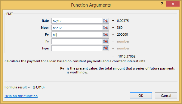
On the Formulas menu select the drop-down “Financial” and then select the PMT function. The wizard pops up:

Use the cursor to select the “rate.”,“nper” (loan term), “Pv” (“present value” or loan amount). Notice that you have to divide the interest rate by 12 since interest is calculated monthly. Also you need to multiply the loan term in years by 12 to get the loan term in months. Press “OK” to save the result in the spreadsheet.

Notice that the payment is shown as a negative number: -1013.37062. To make it positive and add it to the monthly expenses, point to the mortgage cell (E2). Type “=-” then use the cursor to point to the payment field. The resulting formula is =-B4.

Now the spreadsheet looks like this:

Your monthly expenses are $1,863 – Ouch!

Example: Text Function

Here we demonstrate how to use functions inside a formula and text functions.

Suppose you have a list of students as shown below. The first and last name is in one field separated by a comma. We need to put the last and firm names into separate cells. How do we do this?

To tackle this problem you need to use an algorithm – i.e., a step-by-step procedure for doing this.

For example, look at “Washington, George.” The procedure to split that into two words would be:

1. Calculate the length of the string.
2. Find the position of the comma (this shows where one word ends and the other begins).
3. Copy the left-hand side of the string up until the comma.
4. Copy the right-hand side of the string from the comma to the end.

Let’s discuss how to do this with “George Washington” step-by-step in Excel.

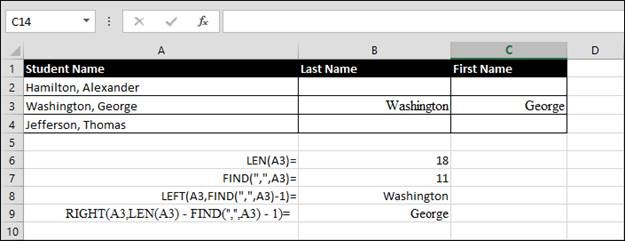
1. Calculate the length of the string with the function =LEN(A3) – the result is 18.
2. Now find the position of the comma by entering this function =FIND(“,”,A3”) – the result is 11.
3. Now take the left-hand side of the string up until the comma and create this nested formula using the result from Step 1: =LEFT(A3,FIND(“,”,A3)-1). Note, we have to subtract 1 from the length because FIND gives the position of the comma.

Here is what that all looks like when all the functions are placed together in a formula. In cell B3, you can see this formula takes all the information from cell A3 and inputs “Washington” into it.

So we have “Washington,” now we need to get “George.” How do we do this?

Note, that we could have saved the result from Step 1 in a cell by itself, say, B6, then write a simpler formula =LEFT(A3,B6-1). But that uses up one cell for the intermittent step.

1. Remember the position of the comma or calculate it again.
2. Calculate the length of the string.
3. Count the characters from the end of the string to the comma.

Take the number of characters from Step 3 and subtract one to omit the comma and space.

Let’s do this step-by-step.

1. From above, this is =FIND(“,”,A3”)
2. The length of the string is =LEN(A3)
3. You will need to use some math to find the number of characters to take: =LEN(A3) – FIND(“,”,A3) – 1
4. The right-hand side of the string we want is =RIGHT(A3,LEN(A3) – FIND(“,”,A3) – 1)

Your spreadsheet should now look similar to the screenshot below. We copied the formulas as text into the bottom of the spreadsheet to make it easier to read and see.

That one was a little difficult but you only need to write these formulas once.